

gprMax is an FDTD solver for ground-penetrating radar. Looking at what it produces meant editing a text file, re-running the solver from a terminal, and running a matplotlib script that decided for you what to show.
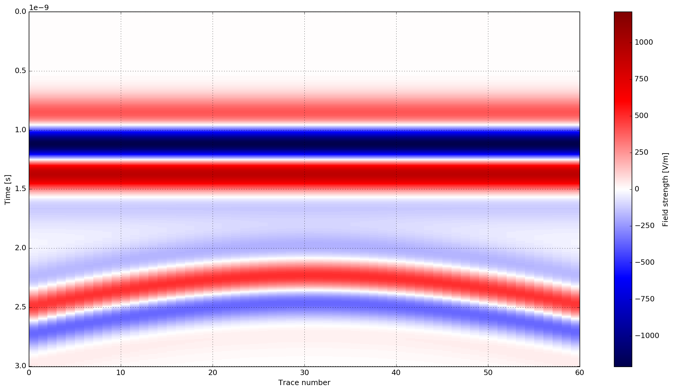
What plot_Bscan.py gives you: one static figure, trace number on the horizontal axis, no processing, nothing to adjust without editing the script and running it again.
This project replaced that loop with six reactive marimo notebooks and four pure-Python modules: a parameter editor with a live geometry preview, a progress tracker, interactive post-processing for A-scans and B-scans, and two notebooks that combine them.
Along the way it turned up three bugs in gprMax’s existing plotting and progress code, and a limit of hyperbola velocity analysis that the tooling now states rather than hides.
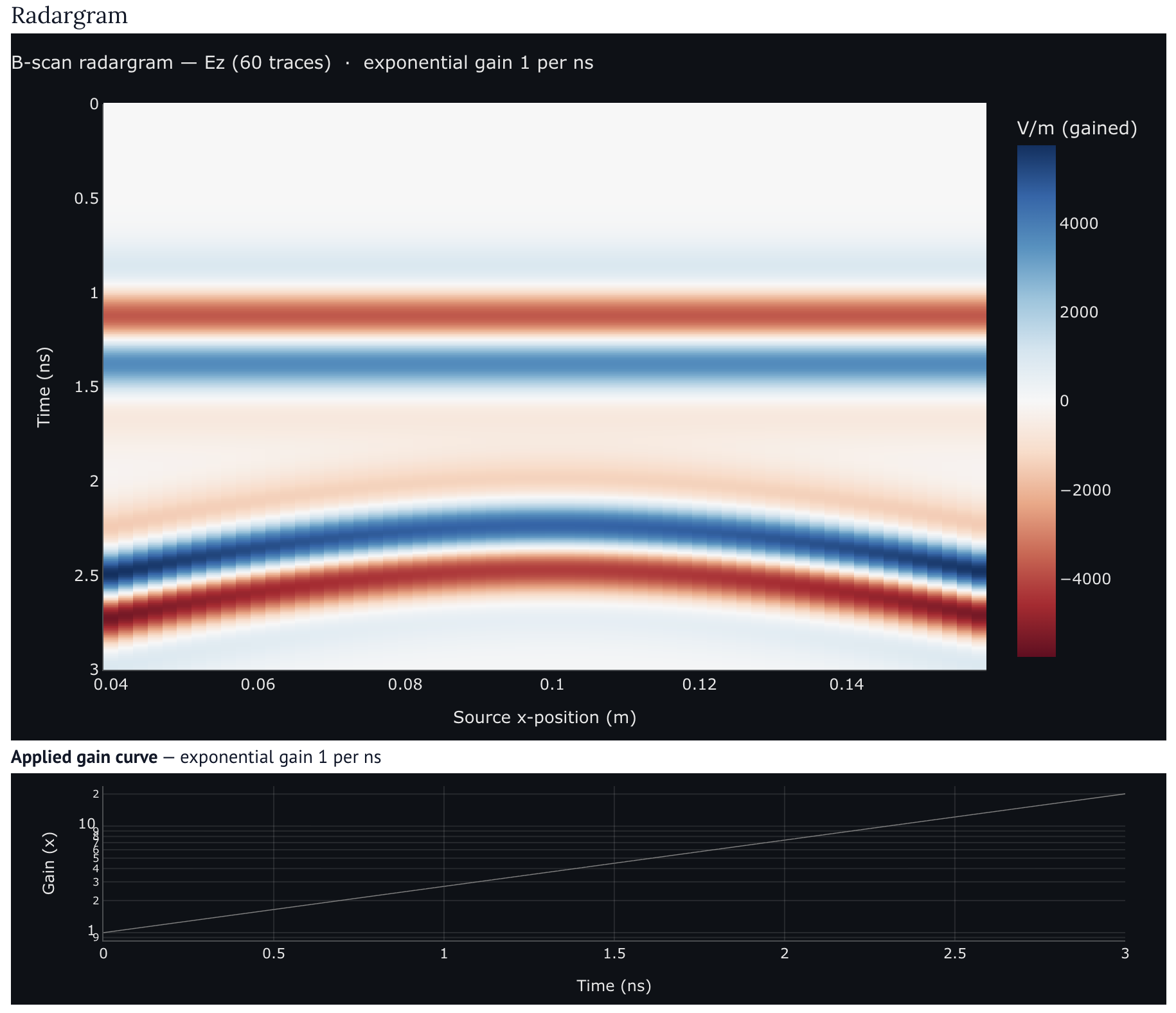
A 60-trace radargram of a metal cylinder buried in a dielectric half-space, exponential gain applied. The hyperbola is the cylinder; the flat bands above it are the direct wave between the two antennas. The panel underneath is the gain curve that was applied, which is the difference between a plot you can read and a plot you have to trust.
What was built
Everything lives in toolboxes/Marimo/. Four files have no marimo import at all, which is the decision the rest of the project rests on: it keeps every piece of real logic testable with plain pytest and usable from an ordinary script.
| Module | |
|---|---|
h5_reader.py |
Reads gprMax v4 HDF5 output into a structured dict. Multi-file loading, filename collisions, every receiver and component, three time-axis units. |
trace_matrix.py |
Validates and stacks single-trace files into an (n_samples, n_traces) radargram, skipping bad files with a recorded reason instead of failing the assembly. |
processing.py |
Gain in six forms, mean-trace background removal, free-space subtraction, FFT. Every function works identically on one trace and on a whole matrix. |
hyperbola.py |
Two-way travel time to a buried target, forwards and backwards, handling the bistatic antenna offset, the target radius and the source waveform delay. |
| Notebook | |
|---|---|
parameter_controls.py |
Sliders driving a live .in preview and a 2D geometry view. |
progress_tracker.py |
Launches gprMax as a subprocess and shows live iteration progress. |
ascan_dashboard.py |
Multi-file workspace, dynamic component selection, dual-axis overlay, free-space subtraction, gain, FFT, export to CSV, SVG, PDF and HTML. |
bscan_dashboard.py |
Radargram from a live directory watch or a finished run, heatmap and 3D surface, gain and background removal. |
recipes/ascan_workflow.py |
Parameters, input file, solver run and waveform in one notebook, with arrival times predicted before the solver starts. |
recipes/velocity_permittivity.py |
Predicted hyperbola overlaid on a real radargram, with permittivity recovered from the measured apex. |
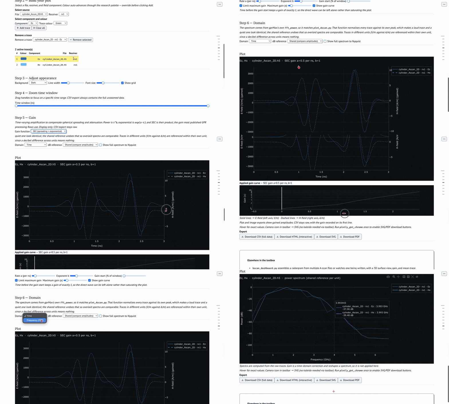
The A-scan dashboard. Traces are added one at a time from any file, receiver and component, and every control re-runs only the cells that depend on it.
Gain, and showing what it did
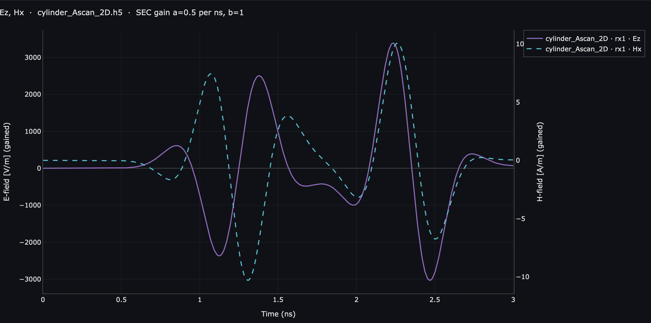
Ez and Hx from the same run, SEC gain applied to both. E-fields and H-fields get separate axes, since V/m and A/m do not belong on one scale.
Six gain functions: constant, linear, power t^b, exponential exp(a·t), dB per ns, and SEC exp(a·t)·t^b, which is the one most published GPR processing uses. The same function applies to a single trace and broadcasts across a whole radargram, so the two cannot drift apart.
The curve that was applied is always drawn underneath the plot. A gained trace on its own tells you nothing about what was done to it, and this was the mentor’s most emphatic request.
Free-space subtraction
Run the model twice, once with the target and once without, and subtract. Everything the two runs share cancels: the source pulse, the antenna coupling, any flat-interface reflection. What survives is the target. In the standard example the cylinder response is about a tenth of the direct wave and hard to pick out. After subtraction it is the largest thing in the trace.
Frequency domain
The transform is gprMax’s own fft_power, imported rather than reimplemented so results match plot_Ascan.py. Two things about that function needed handling at the call site, both described below.
Radargrams, live or after the fact
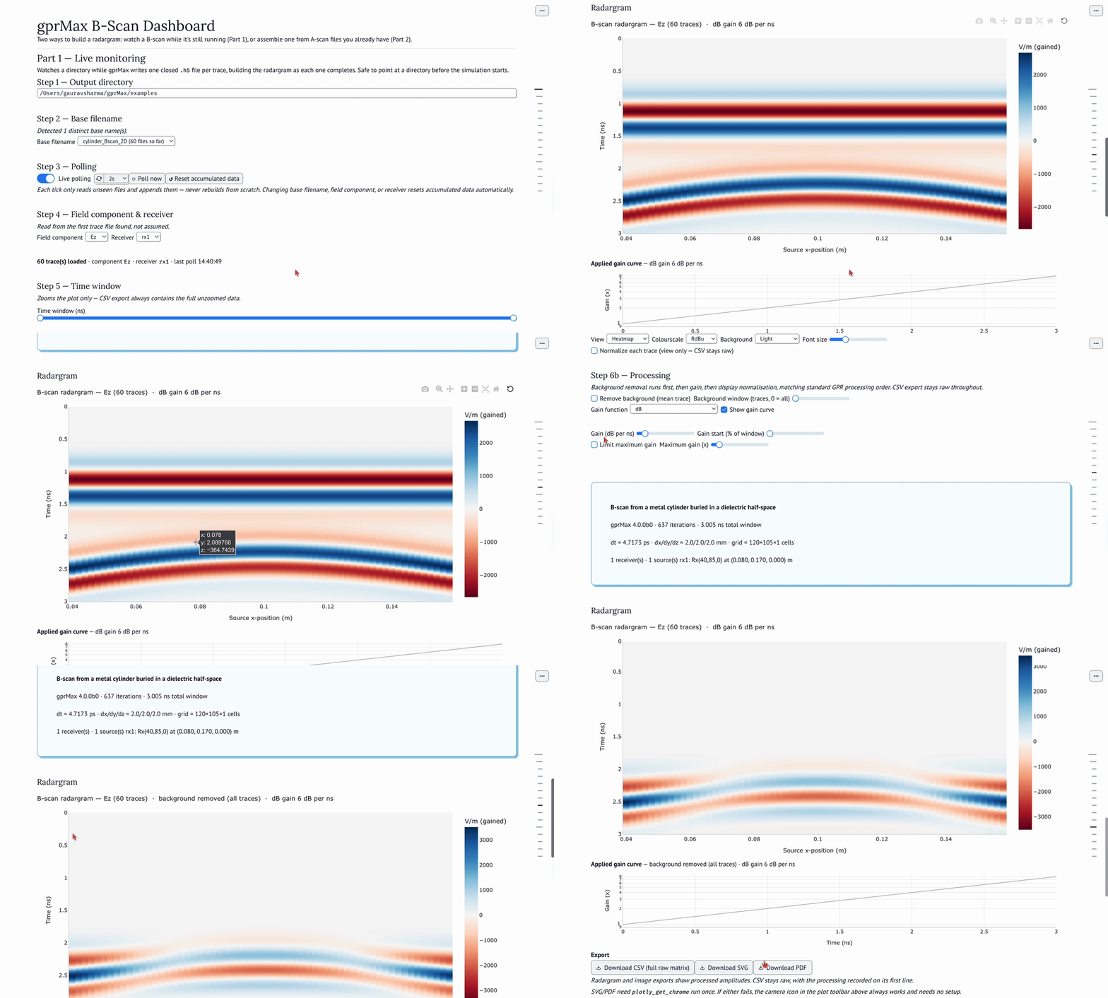
Part 1 watches a directory while gprMax writes one closed file per trace, appending each to the radargram as it lands. Each tick reads only unseen files, so it never rebuilds from scratch.
The same matrix drives a 3D surface, which is sometimes the easier way to see how a reflection changes across the profile.
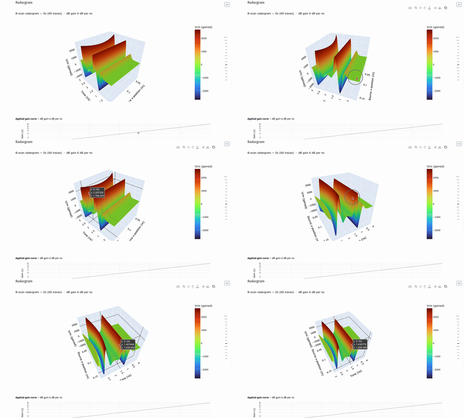
The 3D view and the heatmap are the same assembled matrix and the same processing, drawn two ways.
The recipes
Two notebooks put the pieces together, and both state a physical prediction before showing you the answer.
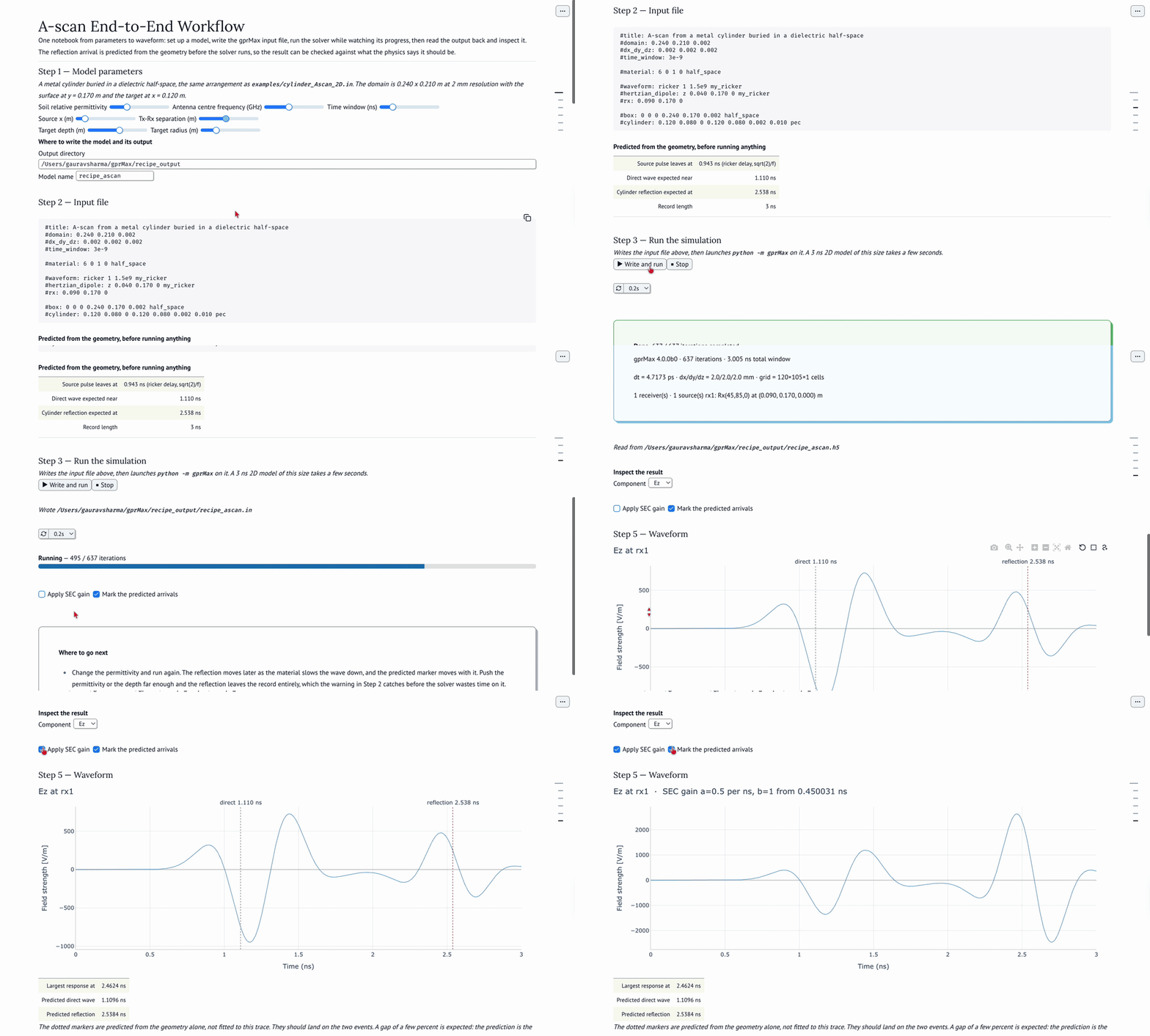
Parameters to input file to solver run to waveform. The arrival times are predicted from the geometry before the solver starts, so the notebook can warn you that a reflection will land outside your time window rather than letting you find out afterwards.
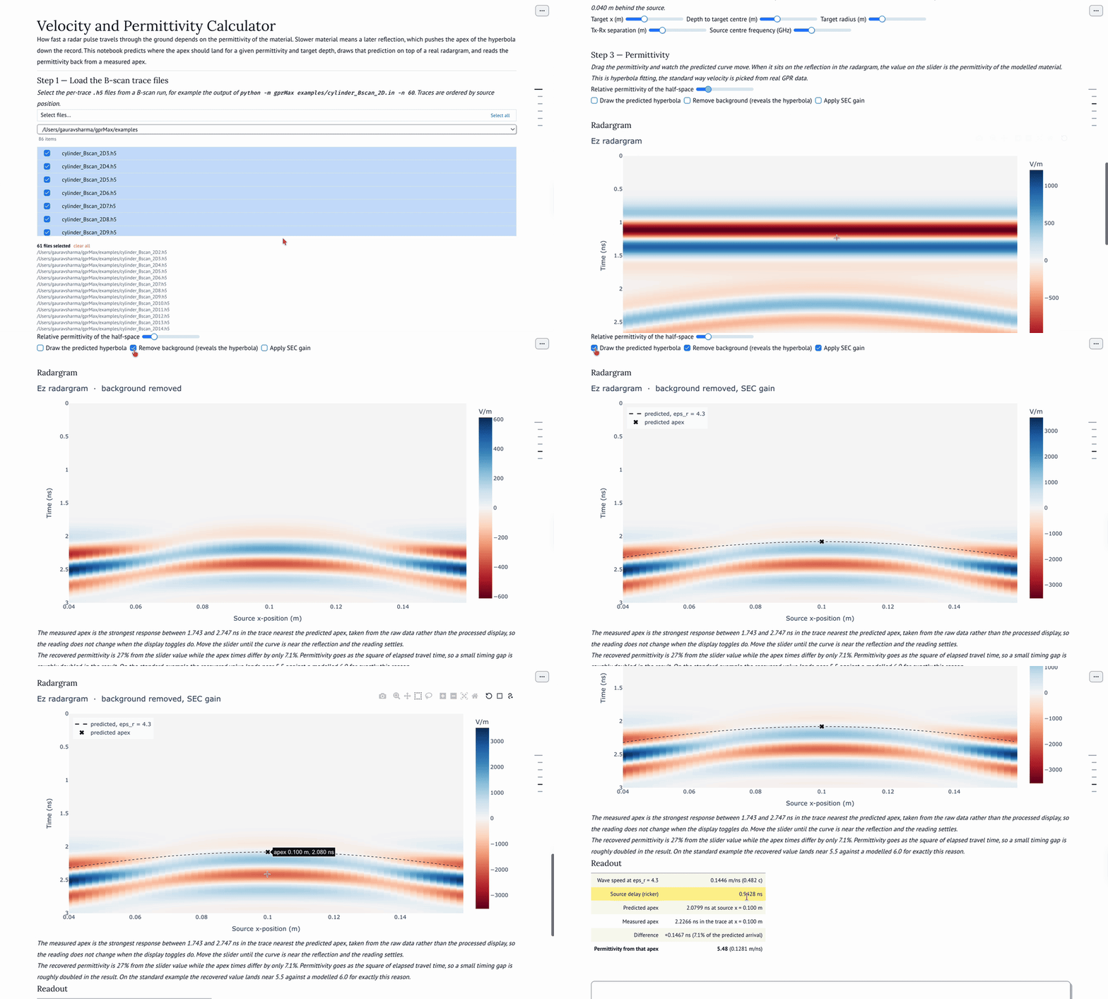
Load a radargram, and the notebook draws the hyperbola a target at a given depth and permittivity would produce. Move the slider until the curve sits on the reflection, and the slider is telling you the permittivity.
Findings
These concern existing gprMax behaviour and stand independently of whether any notebook is merged.
fft_power normalises every trace against its own peak. The last line before it returns shifts the spectrum so its maximum sits at 0 dB. Two traces twenty times apart in amplitude therefore plot identically when overlaid, which quietly defeats the comparison the plot was made for. The dashboard offers a shared reference that recovers the true ratio, computed within each unit family since a decibel difference between V/m and A/m is not a physical statement.
An all-zero trace reaches the same path and produces -inf, which the function’s own guard rewrites to 0, which the normalising shift turns into a flat 0 dB line indistinguishable from real data. Ex in a 2D TMz model is exactly this: stored, never excited. Those traces are now named instead of drawn.
The freqmaxpower * 4 view fallback in plot_Ascan.py is applied as an array index. When the spectral peak sits beyond a quarter of the array it runs past the end. Doing the same thing in frequency and clamping to the available maximum cannot overshoot.
gprMax’s tqdm progress goes to stdout, not stderr. The repository’s own development notes said stderr. Redirecting the two streams separately on a real run returned zero bytes on stderr. There is also no callback or hook API for progress, so parsing the output stream is the only option available rather than a workaround for one.
The ricker source delay is a third of the standard time window. gprMax defines the ricker at t - sqrt(2)/f, so a 1.5 GHz pulse leaves 0.943 ns after the simulation begins, which is 31% of the 3 ns window the standard examples use. Any predicted arrival that omits it is wrong by a third of the plot. It is also not recoverable from the output file, which stores dt, iterations, grid and source position but not the source waveform.
Depth and permittivity cannot be recovered together. Fitting a full twenty-trace hyperbola with the source delay known recovers depth to half a millimetre and permittivity to 0.05. Let the delay float as well, and the same data admits permittivities anywhere from roughly 4 to 7 at sub-picosecond residual. The velocity recipe takes depth as an input, and says why.
Background removal biases a picked arrival time. Subtracting the across-trace mean is what makes a hyperbola visible, but over a limited aperture the moving reflection does not average out, so the mean carries a smeared copy of it. On the standard 60-trace example this pulls the picked apex 0.045 ns early and reports a permittivity of 5.6 against a modelled 6.0. Reading from the raw traces gives 6.02. Every readout in the toolbox processes for display and measures from raw data.
marimo behaviour
Confirmed by running rather than reading documentation. Several of these do not show up in marimo check.
- Reading a widget’s
.valuein the cell that creates it raises at runtime. The static checker misses it. - A cell that writes state and also depends on a widget built from that state never finishes rendering, with no error message. Found by timing a headless export and noticing it never returned.
mo.download’sdataparameter accepts a zero-argument callable. Pass bytes directly and the export is computed on every re-render, which for kaleido means spawning headless Chrome on every timer tick.mo.ui.sliderdefaults todebounce=False;mo.hstackdefaults tojustify="space-between".- Any control whose range is derived from the loaded data is rebuilt, and therefore reset, whenever that data changes.
Validation
The B-scan work was checked against a real 60-trace run of cylinder_Bscan_2D.in on gprMax 4.0.0b0, numerically rather than by eye.
The direct wave arrives at 1.113 ns in every trace with zero spread, which is correct: source and receiver step together with a fixed 0.04 m separation, so nothing shifts the direct coupling. The cylinder reflection moves monotonically from 2.486 ns to 2.227 ns as the source advances, and the hyperbola turns over at source x = 0.100 m, the predicted position, since the cylinder sits at x = 0.120 m and the antenna midpoint trails the source by half the 0.040 m separation.
The analytic model reproduces those arrivals to within about 4%, arriving slightly late. That gap is not removable and is not a modelling error to tune away: the model gives the geometric arrival of an idealised impulse off the nearest point of the target, while the measurement is the peak of a finite-bandwidth wavelet that has propagated through a dispersive FDTD grid.
One consequence is worth recording. Permittivity goes as the square of elapsed travel time, so a 2.6% error in a picked arrival becomes an 8.6% error in the recovered permittivity. Hyperbola fitting is about twice as sensitive as the timing pick it rests on, which is a limit of the method rather than of this implementation.
Tests
| Tests | Statements | Coverage | |
|---|---|---|---|
test_h5_reader.py |
47 | 110 | 98% |
test_trace_matrix.py |
15 | 43 | 98% |
test_processing.py |
68 | 124 | 100% |
test_hyperbola.py |
26 | 48 | 100% |
| Combined | 156 | 325 | 99% |
All against synthetic HDF5 fixtures, so none need a real simulation output or a built gprMax.
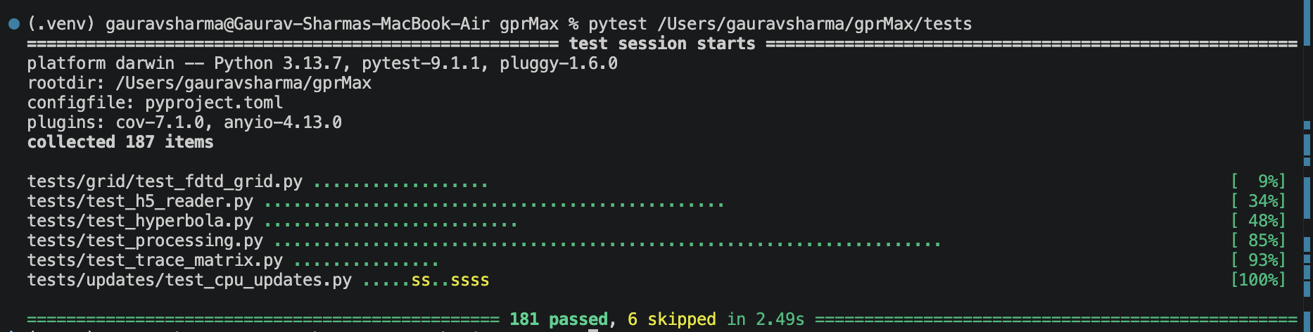
The whole tests/ directory. The four files above account for 156 of these; the remainder, and all six skips, belong to gprMax’s own suite.
The two dashboards measure 0%. A marimo notebook is a marimo.App object with @app.cell functions and no importable surface for pytest to reach, which is the reason for splitting the logic into modules in the first place.
Guards are mutation-tested rather than assumed. Removing the gain broadcast axis, the negative-gain clip, the power floor, the moving-window edge clamp, the subtraction time-step check, the target radius correction or the bistatic apex offset each causes at least one named test to fail.
Pull requests
All against gprMax/gprMax:devel.
| PR | Contents |
|---|---|
| #605 | Three bug fixes in setup.py, found while installing before the coding period |
| #686 | Component 1, parameter controls |
| #696 | Component 3a, A-scan dashboard and h5_reader.py |
| #711 | Component 2, progress tracker |
| #720 | Component 3b, B-scan dashboard and trace_matrix.py |
| #795 | Gain, background removal, subtraction, FFT, processing.py |
| #796 | Component 4, recipes and hyperbola.py |
All seven are open and none has been merged.
Review happened in conversation rather than on GitHub. On the 29 July call Prof. Giannopoulos said he would rather see short messages with screenshots and confirm things verbally than read diffs, and that is how it worked: screenshots to Zulip as each piece landed, and the entire post-midterm scope came out of two calls with him. The pull requests are the record of what was built, not the channel it was reviewed through.
The later PRs are stacked. Each depends on modules from the one before, none of which are merged, so every branch after the first carries its predecessors’ commits into its own diff.
How the scope changed
The proposal described a fairly plain A-scan viewer: read one file, plot Ez, add a range slider.
On 2 July, Prof. Giannopoulos redirected it. What he wanted was a robust foundation for handling the data and options for visualising it, and only then functions that do things to the data. Read as many files as needed, hold the information so the user can plot as they choose, and give them an active element for picking a component from the many read from file.
That turned the design from a funnel, load then pick then plot, into a workspace where everything loads up front and traces are picked interactively. It is why h5_reader.py exists at all. It was not in the proposal.
A second call on 29 July added the amplitude processing: gain functions that compose from a single trace onto a whole radargram, with the applied curve displayable. That became processing.py.
Both redirections were right, and both are in what shipped. The consequence is that components arrived out of proposal order, with Component 3 before Component 2 and Component 4 last.
What was not built
Bandpass and lowpass filters, Gaussian noise injection, and B-scan minus B-scan subtraction are all real requests from the 29 July call, ranked behind gain and FFT. They belong in processing.py and would follow its existing shape; subtract_traces already handles two matrices, so the third is UI work only.
The migration algorithm was ranked lowest by Prof. Giannopoulos himself, to be left for the end if time allowed. It was not.
A VTKHDF model geometry viewer inside marimo was his second priority, framed as something he had attempted himself without completing. It was timeboxed and cut when the processing work took the slot. examples/*.vtkhdf is plain HDF5 and opens with h5py, so this is a well-defined next step rather than an open question.
Docker packaging was a proposal deliverable and was not done. A Dockerfile never tested against a real gprMax build, Cython extensions included, would be worth less than this sentence.
The S11 antenna recipe was moved out of scope by Prof. Giannopoulos, who wants antenna outputs kept out of the GPR notebook. The PML tuning recipe was a stretch goal and was cut.
An Apple Silicon setup.py fix works locally but was never submitted as its own pull request. setup.py selects Homebrew’s gcc-15 on macOS, whose fixed stdio.h includes <_bounds.h> from the macOS 26 SDK while the installed Command Line Tools provide MacOSX15.sdk. Forcing Apple Clang with LLVM libomp sidesteps it.
Challenges
The bugs that mattered were invisible to static checking. A clean marimo check does not mean a notebook runs. Two of the worst problems produce either a runtime error or a notebook that never finishes rendering, and the second has no error message at all. Finding it meant timing a headless export and noticing it never returned. After that, every notebook change went through an AST pass asserting the invariants directly: no same-cell value reads, every cell parameter resolves, every slider debounced, every horizontal stack aligned. That check caught four later regressions, two of them in code that had already shipped.
A performance complaint turned out to be an architecture problem. The B-scan dashboard was reloading every couple of seconds. The cause was not rendering. mo.download was being handed eager bytes, so every poll tick spawned headless Chrome twice for exports nobody had clicked. The same pattern had already been copied into the A-scan dashboard before the flaw in it was understood. A working pattern copied forward propagates its defects silently.
Stacked pull requests are awkward and there is no clean answer. Opening the B-scan PR took four attempts, including one opened against the fork’s own devel branch, which had diverged and produced merge conflicts that did not exist against upstream. The tell was a Settings tab in the repository navigation.
Working without code review. Something had to replace it, and what did was validating against real simulation output rather than assumptions: separating stdout and stderr on a real run instead of trusting the notes, checking exported CSV numbers against predicted arrival times, mutation-testing every guard so a test fails when the thing it protects is removed. That habit produced most of the findings above.
What I learned
Almost every real finding in this project came from checking something that had already been written down.
The development notes said progress went to stderr; a real run said otherwise. The obvious reading of fft_power is that it returns a spectrum, and reading it line by line shows it also normalises, which changes what an overlay means. The textbook hyperbola looks like it should fit a gprMax B-scan, and it does not until the source waveform delay is in it, a delay that is not in the output file at all. Each of those cost an hour to check. Not checking would have cost a plausible, wrong result.
The other thing is that a research tool has to be honest about its own limits. It would have been easy to make the velocity recipe report 6.0 by nudging the geometry until it did. It reports 5.5 and explains why, because a tool that quietly tunes itself toward the expected answer is worse than no tool.
Continuing
I intend to keep contributing to gprMax. The near-term items are the filters and noise injection that fit the existing processing module, B-scan subtraction, the VTKHDF geometry viewer, the Apple Silicon build fix as its own pull request, and responding to review on the seven open PRs whenever it comes.
Running the code
git clone https://github.com/gprMax/gprMax.git
cd gprMax
git checkout devel
pip install -e .
pip install -r toolboxes/Marimo/requirements.txt
plotly_get_chrome            # once, for SVG and PDF export

python -m gprMax examples/cylinder_Ascan_2D.in
marimo run toolboxes/Marimo/ascan_dashboard.py
Full setup and usage notes, including a troubleshooting section, are in toolboxes/Marimo/README.md.